FGT Part 2 - A Closer Look to Microarray Technology

Describe the general properties of the complexity of mRNA populations? Why is it important to consider these properties when planning a gene expression experiment

A population of mRNA extracted from a cell contains not just a lots of different RNA species, but also each with different level of expression. Most of the highest expressed genes are housekeeping genes, which are always expressed in high level to maintain cell activity. Other highest expressed genes are the characteristic of the cell, for example, mitochondrial genes are most expressed in metabolically active cells, or developmental pluripotency associated 5A (Dppa5a) in pluripotent cell. Meanwhile, most of the genes have low expression levels, because they are not expressed.

Hybridisation allows RNA expression levels to be measured

So, in an mRNA population, the most abundant molecules will be dominated by several genes. The problem with this is, sometimes the genes that we find or interested in, are expressed in low levels. In gene expression experiment, what we want to do is comparing mRNA populations between samples, and see which gene are expressed differentially. So, we will probably see similar mRNA abundance distribution even in different cells. And with this, we can also see if there are contaminations (because we expect similar trends).

When the change happens in a lower abundance level (compared to the housekeeping genes for example), it will be hard to detect those. This is true especially when dealing with microarray experiment.

Therefore, we must consider giving the right amount of probe in microarray experiment, because giving more probe to microarray increases the intensity level, but also increses the background intensity.

This happens because the basic of microarray is hybridization. So, a probe-set will complement with its target (specific binding). But, even if the array are able to separate those species through its complementary with certain mRNA, non-specific binding will occur randomly. And this non-specific binding will statistically, caused by the most abundant number of mRNA species in the sample, which contribute to overall background. Increasing probe will also increase the chance of non-specific binding. Therefore it limits the detection level of microarray experiment to measure lower level genes.

You cannot put more probe to detect lower expression in microarray, it just increases background. When you want to detect something rare, we can make more probe of that at lower abundance, but when we do that we are also labelling all the other guys which is not interesting, and all give background.

So, one thing to consider is that microarray relies on the balance between specific binding and non-specific binding. Because microarray measure specific signal against a background of non-specific hybridisation. DNA hybridisation kinetics limit the amount of signal that can be obtained from weakly expressed genes. Labelling more probe label does not generally increases detection because common trancsripts always obtain most of the label.

But nevertheless, sometimes we can see a high number of Trancription Factor in an mRNA population, which connected to a genes.

Outline how PMA (Present, Marginal, Absent) calls are generated from Affymetrix!

To probe genes, oligonucleotides of length 25 bp are used (2). Typically, a mRNA molecule of interest (usually related to a gene) is represented by a probe set composed of 11±20 probe pairs of these oligonucleotides. Each probe pair is composed of a perfect match (PM) probe, a section of the mRNA molecule of interest, and a mismatch (MM) probe that is created by changing the middle (13th) base of the PM with the intention of measuring non-speci®c binding.

In Affymetrix Array, each probesets refer to one specific mRNA or genes. These probesets are a set of 25-ish oligonucleotide which complement to specific mRNAs or genes or predicter exons. The probeset pair composed of two types, which are the Perfect Match probe (PM), and mismatch probe (MM). There is only one single nucleotide differences in the MM. The idea is that the PM will only pair with specific-binding, and the MM will pair with non-specific binding. Therefore, the hybridisation intensity of the mismatch probe is subracted from the perfect match probe to get the correct intensity of specific hybridisation.

In Affymetrix array, the resulting hybridisation scanned into an image file (DAT) which then summarized into a CEL file. This CEL file is the average reads of all the probesets. Then, summary algorithm was generated to create two types of information, one is the number of the signal (the intensity) and the other is the probability of confidence that the gene is expressed or a flag.

What does each call tell you about the expression level of a given gene?

The PMA flag indicates confidence that a particular measurement is from the signal (match) and not from the background (mismatch). This is done by comparing the signal between the PM and MM. Basically it just say how many PM value is higher (brighter) than the corresponding MM value. If tou pick a random intensities, it should result in 50%. Then, we use Fisher's rank sign test to generate p-value. And we can use this significance value from PMA calls as threshold of confidence whether it is:

• P = present, high value, real measurement of expression
• M = marginal, intermediate value, probably expressed
• A = absent, small value, no evidence that signal is different from the background

So, standard image analysis results in image value (signal intensity) and the confidence that the value is from the perfect match signal.

Even so, designing mismatches are not so clever because for example, humans have a lot of Single Nucleotide Polymorphisms. The idea of match/mismatch probes could end up not working because the mismatch probe almost hybridises as well as the perfect match probe. Resulting in subtracting both from each other generate no signal, thus leads to false conclusion. Hence, today we use statistical approaches like RMA (quantile normalisation) which only utilise the PM probe.


How could you use a PMA call alongside fold change filtering of gene to identify deferentially expressed genes?

To de®ne a measure of expression representing the amount of the corresponding mRNA species it is necessary to summarize probe intensities for each probe set. Several

Fold change takes the ratio of a gene's average expression levels under two conditions. It is usually calculated as the difference on the log2 scale. 

Let x ij be the log-transformed expression measurement of the i th gene on the j th array under the control (i = 1,⋯, n and j = 1,⋯, m0), and y ik be the log-transformed expression measurement of the i th gene on the k th array under the treatment (k = 1,⋯m1). We define  and  .

Fold change is computed by

(1)

As for the traditional t test, it is usually calculated on the log2 scale to adjust for the skewness in the original gene expression measurements. The t statistic is then computed by

(2)

where  is the pooled variance of x ij and y ik . Comparing (1) and (2), it is obvious that fold change and t statistic are based on two contradicting assumptions. 

The underlying assumption of fold change is that all genes share a common variance (on the log2 scale), which is implied by the omission of the variance component in (1). On the other hand, the inclusion of in (2) suggests that t test assumes gene-specific variances. 

In order for a gene to be flagged as DE, the double filtering procedure would require the gene to have extreme test scores under the common variance assumption as well as under the gene-specific variance assumption. It is analogous to using the intersection of the rejection regions defined by fold change and t statistic.

Assuming a common variance for all the genes apparently is an oversimplification. The assumption of gene-specific variances, however, leads to unstable estimates due to limited replicates from each gene. A more realistic assumption might lie in between the two extremes, i.e., modeling gene variances by a mixture of two components, one being a point mass at the common variance, another being a continuous distribution for the gene-specific variances. Under this mixture variance assumption, a DE gene could have a large fold change or a large t statistic, but not necessarily both. Taking intersection of the rejection regions flagged by fold change and t statistic, as is adopted by the double filtering procedure, might not be the best strategy under the mixture variance assumption.

MAS5 vs RMA
A significant challenge with Affymetrix expression data is to provide an algorithm that combines the signals from the multiple Perfect-Match (PM) and Mismatch (MM) probes that target each transcript into a single value that sensitively and accurately represents its concentration. 

MAS5.0 does this by calculating a robust average of the (logged) PM-MM values [1]; increased variation is observed at low signal strengths and is at least in part due to the extra noise generated by subtracting the MM values from their PM partners [2].

A number of alternatives (e.g. RMA [3]) have been proposed that ignore the MM values, and consequently do not suffer from this source of variation. RMA successfully reduces the variance of low abundance transcripts and has been shown, using controlled datasets in which known quantities of specific mRNAs have been added to a common reference pool, to better distinguish differentially expressed transcripts from those that are unchanging [2–4].

• MAS5 normalises each array independently and sequentially; RMA as the name suggests (robust multi-array) uses a multi-chip model
• MAS5 uses data from mismatch probes to calculate a "robust average", based on subtracting mismatch probe value from match probe value
• RMA does not use the mismatch probes, because their intensities are often higher than the match probes, making them unreliable as indicators of non-specific binding
• RMA values are in log2 units, MAS5 are not (so values are not directly comparable)

Detection calls

In addition to expression summaries, the Affymetrix software also generates a p-score that assesses the reliability of each expression level. This is produced by using a signed rank test to consider the significance of the difference between the PM and MM values for each probeset [9]. Informally, MAS 5.0 can be seen to return two values, the first, an estimate of transcript concentration, and the second, a measure of how much the software 'believes' the first. Of potential confusion is the fact that this value is referred to as the 'detection p-value', and is subsequently used to generate a 'detection call', which flags the transcript as 'Present', 'Marginal' or 'Absent' (P/M/A)

Continue reading FGT Part 2 - A Closer Look to Microarray Technology

FGT Part 1 - Introduction

Today, we have accomplished to sequence genomes from living beings. Well, not all, but at least we have a quite comprehensive sequence for human and mice.

So, does that mean that we know how life works? How living things were encoded by ACGTs?

Well, not really. Sequencing the genome is just the start. What's next is to understand what it means. And, that is what Functional Genomics is all about.

Right now, we are taking new tools to understand what the genome does. We now have high throughput technologies that can generate whole lots of data and allows us to ask genome scale questions. In other terms, we can screen what happens, what changes, in the genome in different conditions. We can ask, "Can we find a gene that's important for process X?"

Truly, discovery in functional genomics is limited and driven by technology development. It drives and limits our ability to ask question in mass scale. And it's what limiting our knowledge right now. So, in this post, I will talk to you about several Functional Genomic Technologies that are available right now, how to use it, and how to handle the data generated.

Microarray Technology (Gene Expression Array) - The Foundation for Functional Genomics

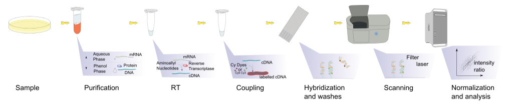
To start with, functional genomic technologies allow us to do large scale measurement of transcription. Suppose you want to identify different genes expressed by human cancer line in response to a drug treatment. So, what you need to do is: (1) treat the cancer cell lines with drug and compare it with untreated one, (2) purify the cells, (3) extract the RNA and make its cDNA/RNA, so, in each tubes we will have ten thousands of RNA molecules. Then, we want to know how many of each different RNA is expressed in comparison with control. 

What we can do is using Microarray technology to do transcriptional profiling. DNA microarray uses collection (library) of DNA spotted in a solid surface, where each spot contains different specific DNA sequence called probes. This probes can be short section of genes or other part of the genome.

First, we couple the RNA samples (target) with labels, which could be a radioactive labels (in the old times) or a fluorescent tags/dye. Then, we hybridize the target with probes. Because of the complementary base pairing, the sample will hybridize with its correct probe pair, and we then wash off the non-specific bindings. Then, using a high resolution image analysis, we can capture the intensity strength of the hybridized probes, and tried to finish the puzzle: (1) which probes expressed differently, and (2) intensity changes: which goes up and which goes down. Then, we can analyse the result summary and statistics. This way, we can make a comparative statement on what is going on in the treated and untreated. 

Overview of DNA microarray process (wikipedia)

Spotted vs Oligonucleotide Microarrays 
The difference between spotted and oligonucleotide microarray is the probe used in analysis. In spotted array, the probes are oligonucleotides, cDNA, or small fragment of PCR product that correspond to mRNA. Oligonucleotide microarrays uses short sequences which are designed to match known or predicted open reading frames.

So, basically, the spotted microarray are more specific and usually used in-house, where it can be modified for each experiments. So, it is better to use spotted microarray if you already know which genes are predicted to change or targeted. Meanwhile, the oligonucleotide can give whole genome results and usually used to screen what is happening in the genome. 

Two-Channel vs One-Channel Detection
There are different ways to label and see the differences between samples: two-channel or one-channel.

In two channel detection, each of the two sample were labelled using different fluorophore dyes (usually its Cy3 and Cy5), mixed together, and hybridized in a single microarray. This way, relative intensities of each fluorophore can be used to analyze up-regulated and down-regulated genes.

In single channel detection, you don't mix it. So it's one microarray per sample. But, this only indicate relative abundance when comparing with different samples. Why? Because each samples will encounter protocol or batch specific bias during amplification, labelling, and hybridization. 

So, looks like its obvious to choose the two channel detection right? Actually it's not. Why? Its because if you want to use multiple comparisons, then you will need more combination for two channel detection while you only need one array per sample using the one channel. And microarrays are still helluva expensive. In conclusion, it is not feasible. 

In fact, one of the most used microarray platform today is the Affymetrix Gene Chip (Hope to make the tutorial too), which is the one-channel detection platform. There are other advantages in using one-channel detection: (1) because each array is exposed to one sample, aberrant sample would not affect raw data of other sample, and it is more flexible to compare with other experiment as long batch effect is accounted for.   

A Rapidly Changing Field: Why You Should Learn Some R Programming

Both strategy would have complication in processing the raw data, but the statistical approach for each platform have been rapidly developed in the recent years. The field was rapidly developing which makes it a bit hard to make a good graphical interface software (it will be outdated a soon as new things published). Rather, people will just upload their code scripts (usually in R language) through open source platform. That is why, basic R language and maybe UNIX command will be necessary to keep updated with this technology. In the coming tutorial, we will use Bioconductor and R to analyze example of Affymetrix data.

The Gene Expression Omnibus (GEO) 
Right now, lots of data has been generated, and they are stored in the gene expression omnibus. Have a look :)

Key Microarray Technologies
Here are some key applicaiton of microarray technology, and we will discuss it more in the next part of this post.

• Expression Arrays (3')
• Probe: cDNA oligo dT primed
• Target: 3' Expressed Sequence Tag (EST)
• Exon Arrays
• Probe: cDNA random primed
• Target: EST / Exon fragments
• Array comparative genomic hybridization (aCGH)
• Probe: Genomic DNA
• Target: Genomic Fragments
• ChIP-on-ChIP / epigenetic modification
• Probe: Affinity purified genomic DNA fragments
• Target: Genomic Fragments
• SNP arrays
• Probe: Genomic allelic variants
• Target: Genomic Sequence
• Protein arrays
• Probe: Antibody/Protein binding protein
• Target: Protein fragments
• Antibody arrays
• Probe: Protein Samples
• Target: Antibodies!

High-Throughput Sequencing (HTS): A Close Relative
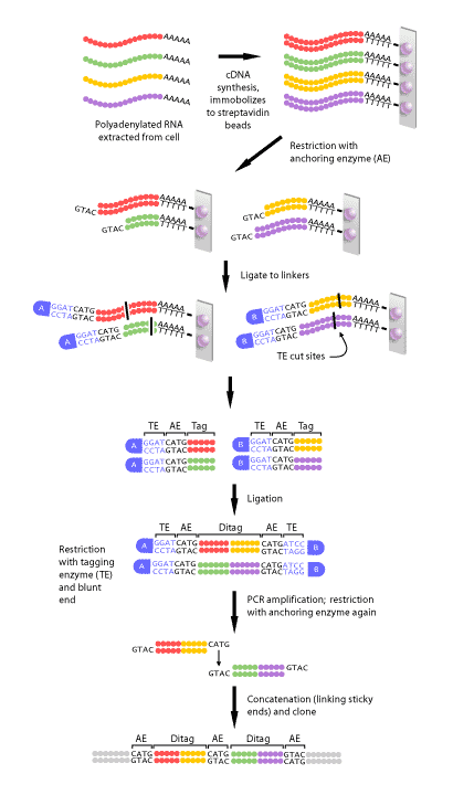
Nucleic-acid based arrays are quite mature, but in the coming years, low-cost high-throughput sequencing technologies will be used as alternative (or replace?) the technique. Some early technologies were Serial Analysis of Gene Expression (SAGE) shown below which basically generates cDNA from RNA population, tags them, and concatenate them for sequencing. Then, we can count the number of cDNA tags and map them to genome. But, we will see some of the newest technology in the next part.

Closing for the First Part
Really, functional genomic allows us to ask genome scale questions, but to make it tell you something biologically relevant, you cannot just relies on statistics alone, it is a combination between measurement and annotation.

Next: Microarray Technologies!

Continue reading FGT Part 1 - Introduction

Kebacut teles, sisanke klebus...

Hai sahabat, 
masih ingat kah di awal 2014, 
ketika sekelompok mahasiswa bandel berkumpul, 
iseng ingin menginisiasi sebuah komunitas baru? 

Entah bagaimana kita berhasil membuat sebuah seminar, tiba2 bergabung menjadi volunteer di acara internasional yang extra ordinary, bermodalkan email bisa sok2 an ke Singapore, dinner bersama para CEO dan berbicara mewakili Indonesia, akhirnya membuat kuliah berseri, dan bisa ngumpul bareng komunitas se-Indonesia di Malang?

Jujur, dengan kondisi yang ada di tempat kita waktu itu, saya cukup pesimis dan bingung untuk melanjutkan apa yang kita mulai. So, saya move on. Mulai memikirkan untuk mencari modal karir, mencari pengalaman "beneran" di lab.

Akhirnya, di MSc ini, saya memilih untuk riset di bawah bimbingan peneliti yang mumpuni sebagai pilihan pertama dan kedua saya. Dengan segala upaya sudah berusaha untuk wawancara dan menulis sebuah draft proposal untuk bisa diterima di pilihan pertama dan kedua ini.

Nah, untuk pilihan ketiga ini, mungkin di hati kecil saya masih ada "unfinished business" dari mimpi yang kita mulai 2 tahun lalu, dan akhirnya saya tuliskan di pilihan ketiga sebuah opsi thesis yang ga biasa, ikutan sebuah lomba.

"Ah, paling keterima di satu atau dua", pikir saya. Tidak seperti pilihan riset, pilihan ketiga ini mewajibkan kami untuk mengirimkan CV. Karena kriteria untuk jadi tim tidak mudah, dan banyak yang berminat, saya kira pilihan ketiga ini justru memudahkan saya untuk mendapat di pilihan sebelumnya. Semacam kalo daftar UGM, pilihan pertama di Biologi, pilihan ketiga di Kedokteran.

Jan, kebacut teles, sisanke klebus...

Entah bagaimana proses seleksinya, ternyata saya malah dapet di pilihan ketiga. Senang, panik, bingung, sedikit kecewa, haha..

Ok guys, sepertinya memang sudah digariskan oleh yang Maha Kuasa untuk menyelesaikan apa yang kita mulai 2 tahun lalu.

Mohon ijin untuk menjadi tim iGEM overgrad Edinburgh, mohon doa restu supaya langkah ini dimudahkan untuk mewakili mimpi dan harapan kita sampai ke Boston smile emoticon

Continue reading Kebacut teles, sisanke klebus...

Kitchen Note - Sambal Terasi!

Ga ada cobek bukan alasan untuk tidak membuat sambal! Tanpa sambal hidup terasa hambar #filosofihidup

Setelah berbulan-bulan mencari resep sambal, akhirnya saya berhasil membuat sambal terasi! #lifeachievement

So, berikut adalah kitchen note dari untuk membuat sambal terasi!

• Garlic (yang banyak, 6-10 siung)
• Shallot (cari yang bulet, 1-2 butir)
• Shrimp Paste (Sainsbury, 1 sendok teh)
• Cabe Ijo (Sainsbury, 3-5 buah, sesuai selera)
• Olive oil
• Tomat (2 buah)
• Oregano (buat tambah2)
• Salt
• HOW TO COOK: Chop everything, panasin wajan (set ke tengah2 panasnya), kasih olive oil, masukin dulu shrimp paste, chopped garlic and shallot, tunggu sampe harum, masukin cabe ama tomat, masak sambil dipenyet2 pake spatula, tambah garam dan oregano sesuai selera

Continue reading Kitchen Note - Sambal Terasi!

Tipe Belajar Paus Terdampar

Tiap orang punya cara belajarnya masing-masing. Entah dari sumber mana, katanya ada orang bertipe visual, audio, by experience, trial and error dll.

Sejak pertama ke UK, entah kenapa saya merasa agak kurang nyaman belajar. Padahal, fasilitas perpustakaan sangat bagus, lab komputer mewah, ada kafe dimana-mana. Tapi, ada sesuatu yang beda dari kebiasaan saya belajar dahulu.

Hari ini, setelah bersih2 kamar (entah sudah berapa minggu ga di bersihin), saya menemukan lagi hal yang "hilang" itu.

Setelah merefleksikan diri, saya sadar bahwa selama lebih dari 10 tahun saya belajar di bangku sekolah, saya lebih sering belajar versi "lesehan" dan "tengkurep". Apalagi ketika kuliah, ketika kerjaan nongkrong di basecamp Kelompok Studi Kelautan, para penghuni Palung "dho pating dlosoran" bagaikan paus terdampar.

Jadi, hari ini saya tumpuk meja belajar saya supaya ruang "dlosor" lebih luas. Ajaibnya, saya merasa lebih produktif!

Ternyata, tipe belajar saya tipe paus terdampar. ‪#‎ajaib‬!

ps: mungkin bisa request ke perpus buat dikasih tempat lesehan, hemat dan murah karena tidak perlu kursi dan meja

Continue reading Tipe Belajar Paus Terdampar

Your Lie in April: A Roller Coaster of Emotions, Amazing Music!

Shigatsu wa kimi no uso (Your Lie in April)

I love classical music

Saya tidak tahu banyak tentang musik klasik, tapi musik klasik sudah mewarnai hidup saya sejak kecil. Maklum, ayah saya seorang dosen dan pemain gitar klasik. Entah di rumah atau di tempat konser (karena diculik nemenin bapak atau dapet tiket gratis), musik klasik bisa memberikan warna yang beraneka ragam di kehidupan kita. Ada sebuah feel yang tidak akan kamu temukan di musik-musik pop di negeri ini.

Itulah alasan pertama saya sangat menikmati seri anime ini.

Saya sudah pernah merasakan duduk di kursi penonton, melihat berbagai macam pertunjukkan klasik yang ada di sekitaran Jogja. Pernah juga saya mengajak beberapa teman kampus untuk melihat konser, dan ada teman yang langsung tidur di beberapa menit pertama (begitu juga di anime ini, haha).

Di anime ini, si mangaka menggambarkan permainan yang sangat menyentuh hati, sampai-sampai ada ilusi yang bisa dilihat si penonton. Agak lebay mungkin. Tapi, kamu akan memahami perasaan itu ketika sudah pernah melihat sebuah pertunjukkan langsung. Pernah di sebuah pertunjukkan musik kontemporer di Pusat Studi Prancis, tiba-tiba suasana menjadi hening, as if the world stopped. Dan ketika kau melihat penonton di kanan kirimu, yang kamu lihat adalah semua orang terdiam, mulut menganga dengan mata berbinar-binar.

That is a moment you'll treasure for your whole life! Really.

Pernah juga waktu itu kami menonton konser dari salah satu pianis kelahiran Indonesia yang sejak kecil tinggal di Belanda (so sorry I can't remember his name!). Di awal pertunjukkan beliau memohon maaf ke penonton karena bahasa Indonesianya yang agak terbatas. Sebuah bakat dan permainan yang luar biasa. Tidak hanya membawakan lagu-lagu klasik dari komposer ternama, beliau juga menampilkan karya original komposisi dia sendiri. I can't stop giving standing applause sampai tangan saya sendiri perih :). Di akhir pertunjukkan, dengan sekeras mungkin berusaha berbicara bahasa Indonesia yang terbata-bata, sang pianis maju ke depan panggung, "Saya mendedikasikan karya terakhir ini untuk kedua orang yang telah menjadikan saya hari ini, yang saat ini duduk di depan saya, ayah dan ibu saya". Sebuah momen yang sangat emosional, yang membuat seluruh penonton memberikan standing applause meskipun si pianis belum memulai permainannya.

Rivalry can always bring you further than you can imagine!

Hmm, setelah saya mengingat-ingat lagi 10 tahun yang lalu, saya meluangkan banyak waktu saya di SMP dan SMA mengikuti kompetisi, yang berawal dari sebuah hom pim pah di depan kampus lama MIPA UGM. Bertemu banyak sahabat baru dan rival baru, telah membawa saya untuk terus memperbaiki diri, sampai bisa melanjutkan studi di UK saat ini. Dan alhamdulillah, silaturahmi itu selalu kami jaga sampai saat ini. Thanks a lot my fiere!

Itulah kenapa saya sangat menikmati tema tersebut di anime ini. I know that feel :)

 "Thank you for giving color to my life" 

Semua orang pasti sudah pernah tau rasanya jatuh, when you can't feel anything, just feeling so negative and down. Mungkin saat itu saya juga merasakan hal yang sama, jenuh dengan segala kesibukan di kompetisi. Just feeling plain, meskipun saat itu sebuah achievement sudah di tangan. Momen ketika hidupmu: monotone.

Then, out of nowhere, a  certain someone come and give a color to my life :)

She is like a roller coaster, a bit selfish and self oriented, yet funny, and beautiful. Dia mungkin menjadi alasanku untuk melanjutkan berkarya, keep me on track. Give me a passion, dan membuatku semakin dewasa. Menang dan kalah tidak lagi menjadi beban, just try your best! Karena ada hal yang lebih berharga untuk diperjuangkan. Kalau dipikir-pikir, kompetisi terakhir yang kami ikuti cuma gara-gara ingin nostalgia di tempat kami dulu bertemu.

Itulah kenapa karakter Kaori di anime ini sangat berkesan bagi saya :)

Dan di sisi lain, I feel so stupid, seperti Kousei yang bener-bener ga sensitif. The one who care about you was always there, so close, yet you don't realise it. But I'm grateful that I'm not too late to realise it :)

But..., Don't watch the series!

Karya ini memang berhak mendapatkan appraisal dari berbagai reviewer. Mungkin banyak komentar juga bahwa karya ini terlalu cliche, tipikal sebuah drama. But..., Don't watch the series if  you're not prepared for the feels!

Awesome music, awesome story.
:)

Continue reading Your Lie in April: A Roller Coaster of Emotions, Amazing Music!

A Reminder of Love, Passion, and the Harsh Truth

Beranjak usia, semakin sering kita melupakan how it feels to be passionate, how it feels to love, how it feels to have a dream. Entah pekerjaan, studi, atau kesibukan lainnya, tampaknya kita semakin sering tenggelam di dalamnya.

Mungkin hal tersebut yang saya rasakan di beberapa bulan terakhir ini, di suasana kuliah yang cukup padat. Tidak hanya itu, dari beberapa diskusi yang kami lakukan di kelas, beberapa peneliti dan dosen senior mulai memberikan pesan,

"Ideas are cheap, what hard is how to make it to the real world. And whether you accept it or not, it's all about who's going to make money out of it at the end. Trust me, I've been an idealist like all of you before"

A bold message. 

Wajah beliau tidak terlihat seakan mematahkan semangat kami, justru menantang kami untuk mengalahkan paradigma tersebut. Tapi, di tengah atmosfer akademisi yang selalu berusaha mencari cela dan celah di paper-paper yang kami baca, rasanya kami hanya menjadi robot untuk mencoba mengkritik ide dan mimpi orang lain.

A heartless robot with a sole purpose to give scrutiny to the work of others. Or is it?

Deep down in our hearts, we know its not true. We were just human. Makhluk ciptaan-Nya yang memiliki hati yang mudah dibolak-balikkan.

So I decided to do something new, a change of atmosphere. Saya belum pernah ke Japanese Film Festival sebelumnya, dan mereka akan screening sebuah film berjudul "5 Centimeter Per Second". Sebuah anime bergenre drama. I'm not a fan of drama, I can't remember the last time I watch a romance drama actually. Tapi, kenapa tidak? Mari kita coba sesuatu yang baru. Toh rating dan review film ini sangat bagus.

Ternyata saya tidak sendirian, ada 2 orang teman Indonesia yang juga tertarik untuk menonton screening film ini. Dan sebagai bonus, ada sushi dari konsulat jendral Jepang di akhir acara, hehe.

Acara dimulai dengan perkenalan dan sedikit penjelasan dari Japanese Literacy Club. "5 centimeter per second... the speed of a cherry blossom falls". Film ini mengambil filosofi dari bunga sakura, cantik dan indah, tapi hanya bisa dinikmati dalam waktu yang sangat singkat. Bangsa Jepang memaknai sakura sebagai simbol dari singkatnya kehidupan. Short and fragile.

Film ini terdiri dari 3 chapter. The first chapter is heartwarming, bagian kedua cukup slow, tapi semua orang menerima bahwa film ini adalah sebuah masterpiece. Bagian ketiga... hmm, this movie is so cruel. A cruel truth and so real, we can refer it to our real world.

5 Centimeters Per Second Trailer HD by pixelentertainment

Seperti kata teman saya, film ini tidak direkomendasikan bagi kamu yang sedang menjalani LDR. But, it is indeed a masterpiece. Makoto Shinkai telah berhasil membuat sebuah karya yang sangat indah secara grafis, dan sebuah emosi yang bisa kita rujuk di kehidupan kita. Meninggalkan sebuah rasa jengkel, kecewa, dan tanda tanya bagi penonton yang sudah selesai menonton film ini. Bukan karena ceritanya jelek (it's a good story, one of the best), tapi mungkin karena kita tidak mau menerima ending dari film ini, which is actually what we really experienced in our real life.

Nevertheless, it makes you think, and re-think about yourself.

Oke, no more spoiler. Selamat menonton!

  

Continue reading A Reminder of Love, Passion, and the Harsh Truth

Practical System Biology Part 3: Belajar Membuat Plot dengan Matplotlib

Hai fellas, kali ini kita akan belajar membuat plot di python dengan menggunakan fitur dari matplotlib. Jika perlu, rekan-rekan bisa menilik lagi postingan saya sebelumnya:

• Part 1: Installing Anaconda, platform untuk Scientific Python
• Part 2: Python Introduction

Kali ini kita akan mencoba mengolah data sebuah eksperimen FISH (fluorescence in situ hybridization). Apa itu FISH? Mari kita bertanya pada wikipedia (opini saya tentang menggunakan wikipedia sebagai sumber ada di bawah):

Singkatnya, kita bisa menggunakan probe berupa potongan salah satu untai DNA yang nantinya akan menempel jika ada pasangan yang komplemen dengan si probe. Nah, dengan demikian, kita bisa mengetahui ada atau tidak sekuen yang kita cari dengan mengukur intensitas fluorosensi dari sel. Data fluorosensi ini diambil dengan menggunakan sensor dari alat seperti Spektrofluorometer (bayangin aja ada kamera lagi nge-video-in sel, terus kita ukur perubahan warnanya dari waktu ke waktu).

Selain bisa nempel di gen yang ada di inti sel (seperti di gambar dari wikipedia), kita juga bisa nempelin si probe ini ke mRNA yang diekspresikan oleh sel. Contoh aplikasi ini bisa dilihat dari video promosi (sumpah ane ga niat marketing) teknologi FISH dari Stellaris:

Dengan demikian, kita bisa mengambil data perubahan jumlah mRNA yang diproduksi sel dari waktu ke waktu.

Exercise Time!

Temen kamu sedang melakukan eksperimen untuk melihat perubahan ekspresi sebuah gen ketika dia memberikan si sel sebuah perlakuan. Untuk itu, temen kamu menggunakan FISH untuk menghitung jumlah mRNA pada sebuah populasi sel setiap enam menit sekali.

Ternyata, data yang dihasilkan dari si alat disimpan dalam format .pkl (pickle) yang merupakan salah satu format untuk bertukar data menggunakan program berbahasa Python. Kamu juga bisa mencari tahu lebih lanjut tentang pickle dengan memasukkan script pickle? di spyder.

Teman kamu meminta tolong untuk mengolah data tersebut menjadi sebuah plot yang mudah dipahami.

Loading data

Hal pertama yang kamu lakukan adalah membuka spyder dan meng-import library yang kita perlukan. Disini kita akan mengimport tiga library: Pickle, Numpy, dan Matplotlib:

import pickle
import matplotlib.pyplot as plt
import numpy as np

Untuk memudahkan mengetik kode, kita singkat matplotlib sebagai plt dan numpy sebagai np. Jadi, selanjutnya teman-teman tinggal menulis plt atau np untuk memanggil fungsi dari masing-masing library. Sementara, save dulu script mu di sebuah folder. 

Memanggil fungsi dari library yang sudah di import

Selanjutnya, kita akan nge-load data dari hasil eksperimen. Pertama, download data FISH, kemudian save di folder yang sama di tempat kamu nge-save script python-mu. Setelah file sudah siap, selanjutnya kita gunakan pickle (how to pickle disini):

d = pickle.load(open('mRNAdata.pkl', 'r'))

Disini, kita mendefinisikan variabel d sebagai data yang akan kita gunakan. 'r' setelah mRNAdata.pkl berarti kita memberikan perintah "read" dari objek pickle. Selanjutnya, yuk kita coba lihat raw data yang kita peroleh seperti apa dengan menulis:

print d

Dan kita peroleh hasilnya ternyata berupa Array yang berisi banyak angka. Di dalam array ini adalah hasil pengukuran intensitas fluorosensi dari 100 sel pada setiap time point. Nah, yg kita perlu lakukan adalah menghitung mean dari 100 sel tadi untuk setiap time point. Dengan demikian, kita bisa membuat plot dengan sumbu x = time points dan sumbu y = rata-rata intensitas fluorosensi dari 100 sel. 

Sek, bentar bro, kok bisa tahu ada 100 sel? Ngitung pake jari satu-satu? Lagian cuma bikin plot pake excel aja mah bisa!

Mencari tahu ukuran data

Nah, inilah kelebihan kita menggunakan Python, kita bisa lebih mudah untuk mengolah data yang berukuran besar. File .pkl yang kita buka tadi ukurannya cuma beberapa kilobyte saja, dan jika kita menghitung secara manual berapa banyak ulangan yang ada di data ini aja udah males :p. Bayangin kalo temen-temen mengolah data genomik yang ukurannya bisa sampai beberapa gigabyte. By the way, kalo filenya besar, fungsi print d tadi bisa membuat laptop kita kewalahan karena harus menampilkan semua data yang ada di dalamnya.

Tampilan data FISH, lingkaran merah menunjukkan sampel intensitas fluorosensi dari 100 sel untuk time point 1, 2, 3, dst. 

So, untuk menghitung ada berapa time points dan jumlah ulangan, kita bisa menggunakan fungsi yang sudah ada di dalam Python (hayo, buka lagi chapter 5!):

ntps= len(d)

atau bisa juga menggunakan modul dari NumPy: 

ntps= np.size(d, axis=0)

Disini kita mendefinisikan variabel ntps (singkatan dari number of time points, atau diberi nama apa aja terserah sih) dengan fungsi len atau np.size (lebih lanjut tentang NumPy). Coba gunakan fungsi print untuk melihat output dari ntps (output = 9).

Nah, untuk melihat ada berapa sampel di tiap time points (ndps = number of data points), kita bisa menggunakan:

ndps= np.size(d, axis=1)

Disini kita menggunakan np.size, tapi kita mengganti axis untuk melihat dimensi di dalam tiap time points.

Teman-teman juga bisa menggunakan fungsi len:

ndps= len(d[0])

Tapi ini hanya untuk melihat dimensi dari timepoints pertama. Coba gunakan fungsi print untuk melihat output dari ndps (output = 100).

Jumlah time points dan ukuran data points

Menghitung Mean dan Standar Deviasi

Untuk membuat plot, kita akan mengukur rata-rata (dm) dari intensitas fluorosensi di tiap time points:

dm= d.mean(axis=1)

dan untuk menghitung standar deviasi (sdm):

sdm= d.std(axis=1)

Dan kita lihat hasilnya:

Rata-rata fluorosensi (merah) dan standar deviasi (biru)

Membuat plot

Nah, data di sumbu Y udah siap nih, sekarang tinggal nyiapin sumbu X, yaitu time points. Dari data, kita sudah tahu bahwa ada 9 time points... artinya apa yak? Artinya, data diambil 9 kali setiap jeda beberapa waktu. Lah, emang jeda waktunya berapa? 6 Menit! (Scroll ke atas deh, yang di highlight dan di bold). Dengan demikian kita bisa tahu data untuk sumbu X:

t= np.arange(ntps)*6

dengan np.arange, kita membuat sebuah array [0, 1, 2, ..., 8], terus tinggal dikali 6 (jeda waktu). Dan kita peroleh:

Selanjutnya, kita akan menggunakan modul dari matplotlib untuk membuat plot. Kita akan menggunakan plt.errorbar() untuk membuat plot dengan error bar. Nah, value dari error bar disini adalah standar deviasi (sdm) dibagi dengan akar dari jumlah sampel (ndps). Kita akan menggunakan NumPy untuk mengakses fungsi square root (np.sqrt). Perhatikan di fungsi plt.errorbar(), t adalah input untuk sumbu X, dm adalah input untuk sumbu Y, dan yerr adalah error bar. Warna dan atribut lain bisa diubah dengan menambahkan argumen seperti ecolor dst. Lebih lengkap di www.matplotlib.org.

plt.figure()

plt.xlabel('time (minutes)')

plt.ylabel('mean mRNA')

plt.errorbar(t, dm, yerr= sdm/np.sqrt(ndps), ecolor= 'k', fmt= 'bo:')

plt.show()

Dan, inilah hasil dari eksperimen teman kita:

Selamat mencoba!

Download script untuk tutorial 3 ini di sini.

Ps: Error bar kecil jadi ga kelihatan, coba kalikan nilai sdm jadi beberapa kali lipat kalau penasaran.

Coming soon: Part 4 - Yuk belajar Entropi!

Continue reading Practical System Biology Part 3: Belajar Membuat Plot dengan Matplotlib

Practical System Biology Part 2: Python Introduction

Nah, bagi teman-teman yang baru pertama kali belajar programming, kita akan menggunakan buku karya Langtangen, “A primer on scientific programming with Python (3rd edition)”. Coba download buku ini dari perpustakaan kampusmu, atau bisa juga didowload dari github sang author (thanks Langtangen!): 
http://hplgit.github.io/primer.html/doc/pub/half/book.pdf.

Untuk belajar, cara paling cepat dan efektif adalah dengan mencoba mengerjakan beberapa exercise yang ada di buku. Kita akan menggunakan chapter 1, 2, 3, dan 5 untuk memahami dasar-dasar Python.

Sebagai panduan belajar, teman-teman bisa mencoba mengikuti saran berikut:

Chapter 1

Bacaan untuk chapter 1:

• 1.1 Pengenalan Python
• 1.2: istilah-istilah di computer science
• 1.3: pembagian dengan integer dan obyek di Python
• 1.4.1: menggunakan modul Python

Latihan untuk chapter 1:

Exercises 1.6 

• Let p be a bank’s interest rate in percent per year. An initial amount A has then grown to:
• 
• after n years. Make a program for computing how much money 1000 euros have grown to after three years with 5 percent interest rate.
• Solution to 1.6

Exercises 1.10

• The bell-shaped Gaussian function, 
• 
• is one of the most widely used functions in science and technology. The parameters m and s > 0 are prescribed real numbers. Make a program for evaluating this function when m = 0, s = 2, and x = 1. Verify the program’s result by comparing with hand calculations on a calculator.
• Solution to 1.10

Chapter 2

Bacaan untuk chapter 2:

• 2.1: while loops
• 2.2: lists dan for loops
• 2.3.1 - 2.3.5: contoh list dan loops
• 2.4: nested lists
• 2.5: tuples
• 2.6.2: contoh aplikasi
• 2.6.3: cara mencari informasi dalam Python

Latihan untuk chapter 2:

Exercise 2.10

• We want to generate x coordinates between 1 and 2 with spacing 0.01. The coordinates are given by the formula xi = 1 + ih, where h = 0.01 and i runs over integers 0, 1, . . . , 100. Compute the xi values and store them in a list (use a for loop, and append each new xi value to a list, which is empty initially).
• Solution to 2.10

Exercise 2.12 

• The following code is supposed to compute the sum function:
• 
• s = 0; k = 1; M = 100
• while k < M:
• s += 1/k
• print s
• This program does not work correctly. What are the three errors? (If you try to run the program, nothing will happen on the screen. Type Ctrl+c, i.e., hold down the Control (Ctrl) key and then type the c key, to stop the program.) Write a correct program.
• Hint. There are two basic ways to find errors in a program: (1) read the program carefully and think about the consequences of each statement, (2) print out intermediate results and compare with hand calculations. First, try method 1 and find as many errors as you can. Thereafter, try method 2 for M = 3 and compare the evolution of s with your own hand calculations.
• Solution to 2.12

Exercise 2.13

• Rewrite the corrected version of the program in Exercise 2.12 using a for loop over k values instead of a while loop.
• Solution to 2.13

Chapter 3

Bacaan untuk chapter 3:

• 3.1.1 - 3.1.6: functions
• 3.1.10: the main program
• 3.2: branching and if statements
• 3.3.1: using functions

Latihan untuk chapter 3:

Exercise 3.1

• The the formula above is for converting Fahrenheit degrees to Celsius reads.
• Write a function C(F) that implements this formula. To verify the implementation of C(F), you can convert a Celsius temperature to Fahrenheit and then back to Celsius again using the F(C) function from Chapter 3.1.1 and the C(F) function. That is, you can check that the boolean expression c == C(F(c)) is True for any temperature c (you should, however, be careful with comparing real numbers with ==, see Exercise 2.24).
• Solution to 3.1

Exercise 3.4 

• The standard Python function called sum takes a list as argument and computes the sum of the elements in the list:
• >>> sum([1,3,5,-5])
• 4
• Implement your own version of sum. 
• Solution to 3.4

Exercise 3.14 

• Make a Python function gauss(x, m=0, s=1) for computing the Gaussian function 
• 
• Call gauss(x) and print out the result for x ∈ [−5, 5] (say for 11 uniformly spaced x values). 
• Solution to 3.14

Exercise 3.23

• Given a list a, the max function in Python’s standard library computes the largest element in a: max(a). Similarly, min(a) returns the smallest element in a. The purpose of this exercise is to write your own max and min function. Use the following technique: Initialize a variable max_elem by the first element in the list, then visit all the remaining elements (a[1:]), compare each element to max_elem, and if greater, make max_elem refer to that element. Use a similar technique to compute the minimum element. Collect the two pieces of code in functions.
• Solution to 3.23

Exercise 3.34

• Write a function count_pairs(dna, pair) that returns the number of occurrences of a pair of characters (pair) in a DNA string (dna). For example, calling the function with dna as ’ACTGCTATCCATT’ and pair as ’AT’ will return 2. 
• Solution to 3.34

Chapter 5

Bacaan untuk chapter 5:

• 5.3.1 - 5.3.2: plotting data
• 5.6.1: arrays
• 5.6.4: accessing elements of arrays
• 5.6.7: manipulating the shape of arrays
• 5.7.1 - 5.7.2: arrays with more than one dimension

Nah, setelah mencoba latihan-latihan diatas, teman-teman pasti sudah lebih familiar dengan Python.

Loh, ga ada latihan untuk Chapter 5 nih??

Jangan khawatir, di postingan selanjutnya, kita akan mencoba belajar membuat plot dengan menggunakan contoh Fluorescence In Situ Hybridization (FISH).

Next, Part 3: Membuat Plot dengan Python dan MatPlotLib

Continue reading Practical System Biology Part 2: Python Introduction